How To Change Line Width In Matlab

Introduction to Matlab LineWidth

At that place are the various operations of lines in Matlab in which line width is one of the operations. Line width is used to adjust (increase) the width of any object. Line width performance mostly executes inside the plot operation. Plot operation is used to plot the input and output in a graphical way. We tin increment the width of an object to whatsoever extent. By default, the line width size is 'ane' in Matlab. Sometimes in complex figures or diagrams output gets disturbed or vanish, in such cases line width plays an important role. This control is represented every bit 'LineWidth'. In this topic, we are going to acquire about Matlab LineWidth.

Syntax –

Plot( x axis values, y axis values, 'LineWidth', value of width)

Example – plot(x,y,'LineWidth',ane)

How does Matlab linewidth piece of work?

Algorithm to implement LineWidth control in Matlab given below;

Step one: Accept ii inputs to plot graph

Step two: Plot the graph

Footstep 3: Utilise line width control

Pace iv: Brandish the consequence

Examples

Here are the examples of Matlab LineWidth mention below

Instance #1

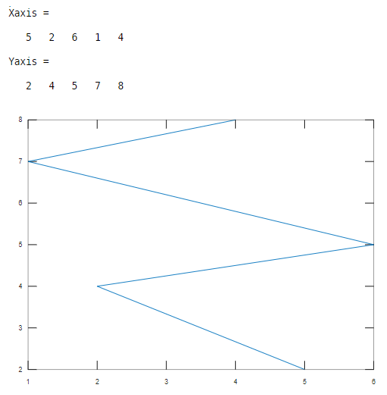
Let usa consider ii inputs every bit x-axis and y-axis. Here the values of first input are 5, 2, 6,i,4 and values of second input are 2,four,5,7,8. And the line width value is ane. This example illustrated in table 1.

Code:

Xaxis =[ 5 ii six 1 4] Yaxis =[2 4 five 7 8 ] plot(Xaxis , Yaxis ,'LineWidth', ane)

Output:

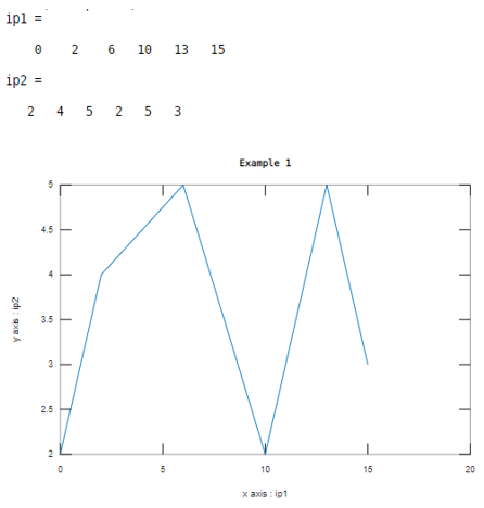
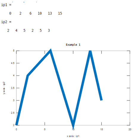
Let us consider ii inputs as xaxis and yaxis. Here values of  offset input are  0, 2 , half dozen , i 0 , one 3 , 1 5  and values of second input are 2 , 4 , 5 , 2 , v , 3 . And the line width value is 1. This example illustrated in table ii.

Code:

ip1=[ 0 2 six ten 13 15] ip2=[2 4 v 2 5 iii] xlabel('x axis : ip1');
ylabel('y axis : ip2');
plot(ip1 ,ip2,'LineWidth',one)
championship('Instance 1')

Output:

Example #2

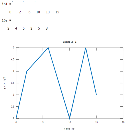
Let u.s.a. consider two inputs as xaxis and yaxis. Here values of  first input are  0, 2 , 6 , i 0 , 1 three , one 5  and values of second input are 2 , 4 , 5 , ii , 5 , three . And the line width value is iii. This example illustrated in table 3

Code:

ip1=[ 0 ii 6 10 13 15] ip2=[2 4 five 2 five 3] xlabel('ten axis : ip1');
ylabel('y axis : ip2');
plot(ip1,ip2,'LineWidth',3)
title('Case one')

Output:

Example #3

Let us consider two inputs equally xaxis and yaxis. Here values of  start input are  0, 2 , 6 , 1 0 , ane 3 , 1 5  and values of second input are 2 , four , 5 , 2 , 5 , iii . And the line width value is x. This example illustrated in tabular array 3

Code:

ip1=[ 0 2 6 x thirteen fifteen] ip2=[2 4 5 2 5 iii] xlabel('10 axis : ip1');
ylabel('y centrality : ip2');
plot(ip1,ip2,'LineWidth',10)
title('Instance one')

Output:

Example #four

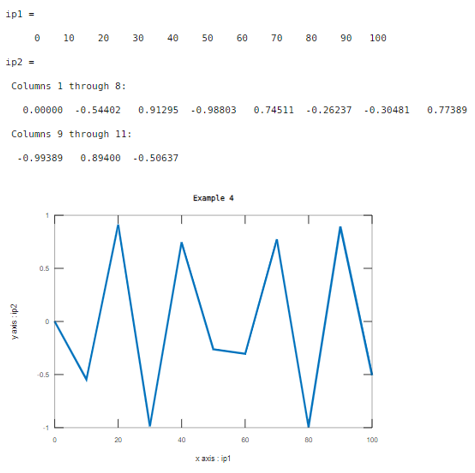
Let us consider two inputs as xaxis and yaxis. Hither the values of first input are range betwixt  0 to 100 with a step of 10  and the values of 2nd input are sine function. And the line width value is 3. This instance illustrated in tabular array 4

Code:

ip1=0:10:100
ip2=sin(ip1)
xlabel('10 centrality : ip1');
ylabel('y axis : ip2');
plot(ip1,ip2,'LineWidth',3)
title('Example 4')

Output:

Example #5

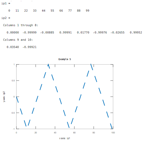
Let us consider two inputs as xaxis and yaxis. Hither the values of start input are range between 0 to 100 with a stride of 10  and the values of 2d input are sine role. And the line width value is iii. The difference between the previous examples and this example is the pattern of width. This case illustrated in table 5.

Code:

ip1=0:11:100
ip2=sin(ip1)
xlabel('x axis : ip1');
ylabel('y axis : ip2');
plot(ip1,ip2,'--','LineWidth',3)
title('Case v')

Output:

Instance #6

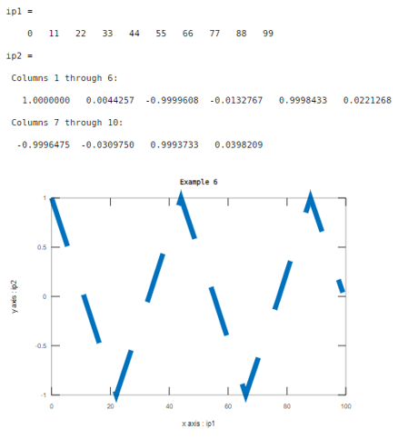
In this instance, the first input is a range of values from 0 to 100 with the step of 11. And the second input is the cosine signal with respect to the kickoff input. Here line width is 8 and the blueprint is dash lines.

Code:

ip1=0:eleven:100
ip2=cos(ip1)
xlabel('x axis : ip1');
ylabel('y centrality : ip2');
plot(ip1,ip2,'--','LineWidth',8)
championship('Instance half-dozen')

Output:

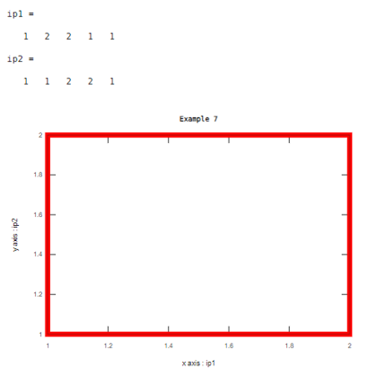
Case #7

In this example, the output is i object which is a rectangle. Line width is eight and the color of width is ruby-red which we need to declare in program .otherwise default colour is blue similar previous examples.

Code:

ip1=[one ii 2 1 i] ip2=[1 one ii two i] xlabel('x centrality : ip1');
ylabel('y axis : ip2');
plot(ip1,ip2,'LineWidth',8,'color','red')
title('Example vii')

Output:

Conclusion

If the output of the program is a specific object so line width plays an important role, it gives proper view to object .line width is basically used to increase the thickness of width line .along with thickness we can change the color of width and pattern of width.

Recommended Articles

This is a guide to Matlab LineWidth. Hither nosotros hash out the algorithm to implement LineWidth control in Matlab along with the examples and outputs. You lot may also take a look at the following articles to larn more –

1. Arrays in Matlab
2. 3D Plots in Matlab
3. Matlab Create Function
4. Loops in Matlab
5. Complete Guide to Reshape in Matlab
6. Examples of xlabel Matlab

Source: https://www.educba.com/matlab-linewidth/

Posted by: henrypeargen.blogspot.com

Share this post